Neural Networks

MGMT 638: Data-Driven Investments: Equity

Kerry Back, Rice University

{height=380 width=760 fig-align="center"}

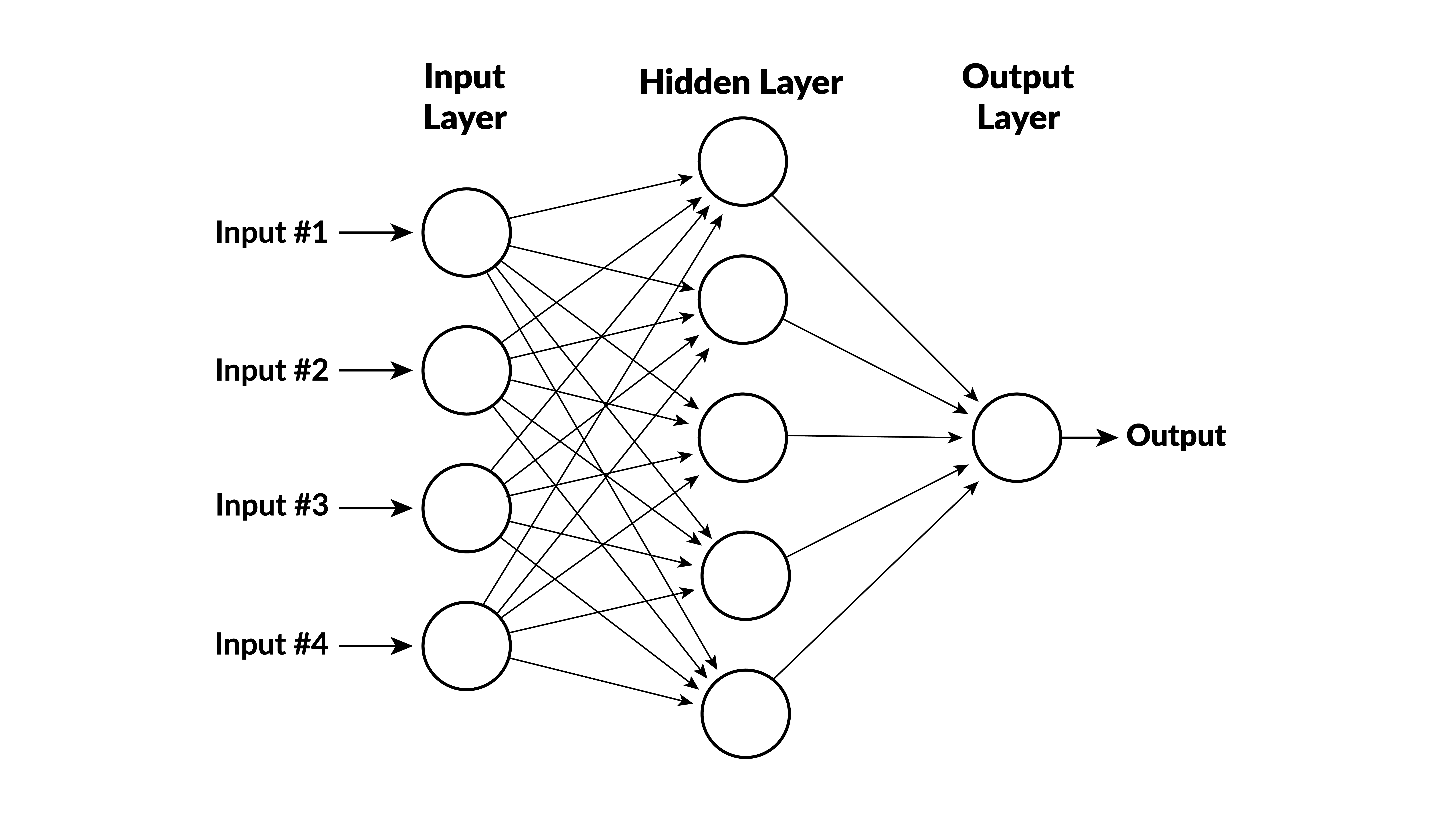
• inputs $x_1, x_2, x_3, x_4$
• variables $y_1, \ldots, y_5$ are calculated in hidden layer
• output depends on $y_1, \ldots, y_5$

Rectified linear units

• The usual function for the neurons (except in the last layer) is

. . .

$$ y = \max(0,b+w_1x_1 + \cdots + w_nx_n)$$

• Parameters $b$ (called bias) and $w_1, \ldots w_n$ (called weights) are different for different neurons.
• This function is called a rectified linear unit (RLU).

Analogy to neurons firing

• If $w_i>0$ then $y>0$ only when $x_i$ are large enough.
• A neuron fires when it is sufficiently stimulated by signals from other neurons (in prior layer).

Output function

• The output doesn't have a truncation, so it can be negative.
• For regression problems, it is linear:

$$z = b+w_1y_1 + \cdots + w_ny_n$$

• For classification, there is a linear function for each class and the prediction is the class with the largest value.

Imports

from sklearn.neural_network import MLPRegressor
import numpy as np
import pandas as pd
import matplotlib.pyplot as plt 
import seaborn as sns
sns.set_style("whitegrid")

Generate data

np.random.seed(0)
x1 = np.random.normal(size=1000)
x2 = np.random.normal(size=1000)
e = np.random.normal(size=1000)
y = 2*x1 + 3*x2 + e
df = pd.DataFrame(
    dict(x1=x1, x2=x2, y=y)
)
df.head()

	x1	x2	y
0	1.764052	0.555963	3.663072
1	0.400157	0.892474	1.765766
2	0.978738	-0.422315	0.736667
3	2.240893	0.104714	3.837554
4	1.867558	0.228053	4.338464

Fit a neural network

net = MLPRegressor(
    hidden_layer_sizes=[8, 8, 4],
    solver="adam"
)
net.fit(X=df[["x1", "x2"]], y=df.y)

c:\Users\kerry\AppData\Local\Programs\Python\Python310\lib\site-packages\sklearn\neural_network\_multilayer_perceptron.py:702: ConvergenceWarning: Stochastic Optimizer: Maximum iterations (200) reached and the optimization hasn't converged yet.
  warnings.warn(

MLPRegressor(hidden_layer_sizes=[8, 8, 4])

In a Jupyter environment, please rerun this cell to show the HTML representation or trust the notebook.
On GitHub, the HTML representation is unable to render, please try loading this page with nbviewer.org.

View goodness of fit

predictions = net.predict(X=df[["x1", "x2"]])
sns.regplot(x=df.y, y=predictions, ci=None)
df = df.sort_values(by="y")
plt.xlabel("Actual y")
plt.ylabel("Predicted y")
plt.show()